Entries tagged as mathematics
Wednesday, December 30. 2015
Vehicle production cost vs. efficient fuel usage

I recently read[1] that 10% of the energy an automobile consumes during its lifetime already occur during production, i.e., only 90% of energy are burnt fuel. This made me wonder, looking at the option of trading an old car for a new one with a more efficient engine that burns less fuel per distance: When does the saved fuel pay off the production of the second vehicle? (Note that we’re not talking about when the saved fuel pays off financially.)
Let’s make some assumptions for a first guess: The old car burns 0.07 ℓ/km (7 ℓ/100 km) of whatever fuel type. Assuming a lifetime of 8 years with 20,000 km/y, we drive 160,000 km and thus burn 11,200 ℓ of fuel. These are our 90%. Thus, 1,244 ℓ fuel-equivalents of energy are used for production; let’s take pessimistic 1,300 ℓ, because we don’t know whether the production of the new car is more or less energy-expensive than the old one anyway.
The two sides of the equation reflect the two possibilities: Either produce only one car and spend more fuel, or produce two cars, spend some fuel for the first and then less fuel for the second. When should we switch, and for how long should we drive the second car? It turns out that the “when should we switch” is irrelevant, we only have to consider that producing two cars is more expensive than just one, and we have to recover from that difference by saving fuel.
So, we spend 1,300 ℓ production plus 20,000 km/y × years used × 0.07 ℓ/km fuel for the old car. (km⁄y × y × ℓ⁄km = ℓ.) Assume further that the new car only needs 0.06 ℓ/km, what yields 2 × 1300 + 20000 y × 0.06 correspondingly. The equation thus turns into
20000 y (0.07−0.06) = 1300 or y = 1300⁄200 = 6.5,
meaning that switching cars only pays off towards the end of the lifetime of the second car if we only gain 0.01 ℓ/km. If the new car saves twice as much, 0.02 ℓ/km, it takes only half that time, but still 3–4 years. And it’s only until after that time that our economy environment gains some benefit—but still only the saved fuel, not the total, of course.
As a conclusion, it does pay off, but only hardly. The best option is still not to drive (and fly!) that much. And don’t think that electric vehicles are that much better: They still need energy for production and for charging the battery, and the corresponding electric infrastructure has to be scaled up and supplied, demanding even more energy from... where? In addition, and in contrast to fuel, the battery is just an energy carrier, not an energy source, so something is always lost during conversion.
If you have the impression that our industrial society as it is today is doomed, you’re right, sadly. If you don’t have that impression, I recommend you to read this book, even if it’s already ten years old:
Thursday, January 20. 2011
Aftermath in the truest sense, II
One year ago I wrote about that I was authoring a chapter for a book about mathematical imaging together with O. Christensen and H. Feichtinger. Some months ago our contribution was accepted as Chapter 29 (“Gabor Analysis for Imaging”) of Springer’s “Handbook of Mathematical Methods in Imaging” (ISBN 978-0-387-92920-0). The book is available for online access since last week for ~€600. As it has got 1607 pages, it will take me some time to read through it.
As mentioned previously, our content mainly resembles the structure of my Master’s thesis from 2007, but with more mathematical rigor thanks to the two mentioned authors. Originally I wanted to recreate the pictures I had shown in my thesis, but decided to just reuse them.
Sunday, May 2. 2010
Averaging an image sequence with ImageMagick

Besides the fact that it was a pain to find out how ImageMagick’s -average option is to be used, it turned out to operate wrongly. The switch calculates the mean of an image sequence, i.e. the mean color values for every pixel. Say, if you have a bunch of images with file names like img*.jpg and want the average saved into avg.jpg, the command line is:
Pretty intuitive. The problem is that you define the mean image Ī[n] of n images I[k] as
while ImageMagick does it recursively as
(with Ĩ[1]=I[1]),
giving you wrong weights 1⁄2n−k+1 like e.g. for n=8
![]()
instead of the intended weights 1⁄n like
![]() .
.
This misbehaviour can be proven e.g. by taking this sequence of a plain blue, green and red image:
![]()
![]()
![]()
and averaging it with the above command. The result is too reddish:
![]()
The solution I found was to call convert recursively like this:
i=0
for file in img*jpg; do
echo -n "$file.. "
if [ $i -eq 0 ]; then
cp $file avg.jpg
else
convert $file avg.jpg -fx "(u+$i*v)/$[$i+1]" avg.jpg
fi
i=$[$i+1]
done
By this, the average of the above example images correctly becomes gray:
![]()
There might be similar problems with the other image sequence operators, but I haven’t examined them. Maybe I should file a bug.
Saturday, January 16. 2010
Aftermath in the truest sense
Two years have passed since I declared the project “Master’s thesis” accomplished. Continuing with a PhD was already unlikely at that time and became even more unlikely since then. However, O. Christensen, the author of one of my main sources, asked me a few months ago to contribute to a book chapter he was writing together with my advisor, Prof. H. Feichtinger. Parts of my thesis might thus show up in a book about imaging from a major publisher of mathematical works. We submitted our result this week. I won’t tell more at this time, except that it was fun to dig through the material again. It might take a few months until a decision is made by the publisher. Whatever the result, I don’t expect it to lead me back to academia.
Friday, September 4. 2009
Light gain with fast lenses

I was interested what difference there is between the Canon EF 50mm f/1.2, f/1.4 and the f/1.8 model regarding the light gain compared to an f/2.8 lens. The amount of light that travels through an optical system is usually given by f-numbers, the relation between focal length and aperture diameter. Doubling or halving the diameter of the aperture results in quadrupling/quartering the aperture area and thus the amount of light that can fall through:
Practically it is of interest what f-numbers result in doubling/halving the amount of light,
,
what is thus given by an aperture diameter change factor of √2 ≈ 1.41. Continuously doubling/halving the light amount results in the diameter changing with the factors (√2)k, yielding the classical sequence
1.4 → 2.0 → 2.8 → 4.0 → 5.6 → 8.0 → ...
The switch from a lens with maximum f/2.8 to one with f/1.4 thus yields 4× as much light, allowing ¼ of the original exposure time. Between f/2.8 and f/2.0 there’s a factor of 2. So, switching f/2.8 to f/1.8 must gain light with a factor between 2 and 4. What’s the exact amount? It’s
So it’s even less than 2.5, while with an f/1.4 lens it’s a factor of 4! Thus, there’s quite a difference in the light amount between those two lenses. And what about the step from f/2.8 to f/1.2? The gain factor is calculated similarly: 5.44. The step from f/1.4 to f/1.2 only yields 1.36× more light.
Sunday, January 11. 2009
Magic ball volumes in high-dimensional spaces
Currently I’m dealing with the topic of machine learning at work, and I stepped over the so-called curse of dimensionality, where the volume of the unit ball (radius=1) becomes negligible compared to the volume of the unit cube (side length=1) which is always equal to 1, what yields problems when selecting a number of training samples in a (very) high-dimensional feature space. My team-mate and I stepped over an interesting thing concerning the volume of the unit ball in higher dimensions.
First of all, the formula for calculating the volume of the ball Brn ⊂ ℝn with radius r is given as
.
In two dimensions (n=2) we get the volume as the well-known circle area r2π, and as Γ(2.5)=¾√π, we get the ball volume for n=3 as 4⁄3r3π. In higher dimensions the resulting formula isn’t that simple anymore, but we’re only interested in the numerical values anyway. We now restrict to r=1. Following one’s intuition, the volume increases with the dimensions (ball volume is larger than circle area), but see what happens beginning with n=5 and n=13:
| n | V | n | V |
|---|---|---|---|
| 1 | 2 | 11 | 1.88 |
| 2 | π ≈ 3.14 | 12 | 1.34 |
| 3 | 4⁄3π ≈ 4.19 | 13 | 0.91 |
| 4 | 4.93 | 14 | 0.60 |
| 5 | 5.26 | 15 | 0.38 |
| 6 | 5.17 | 16 | 0.24 |
| 7 | 4.72 | 17 | 0.14 |
| 8 | 4.06 | 18 | 0.08 |
| 9 | 3.30 | 19 | 0.05 |
| 10 | 2.55 | 20 | 0.03 |
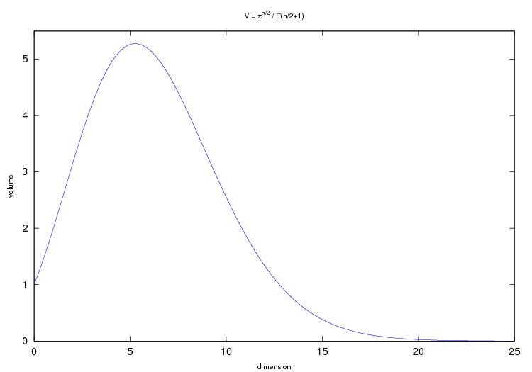
This is indeed interesting: The ball volume starts to decrease and even goes to zero in higher dimensions, although its radius is always 1! What does that mean? And why is the unit cube able to keep its volume of 1, although it seems to be contained within the unit ball? Another thing we see: A bit past n=5 the function reaches its maximum of something a bit larger than 5. Do we have V(x0)=x0 for x0=sup V(x)? And if so, what’s its value?
The key in understanding this issue lies in the corners of the unit cube: Their distance to the origin goes to infinity with increasing number of dimensions! For the unit square (2-cube), their distance is √½ ≈ 0.71, and for the 3-cube it’s already √¾ ≈ 0.87. At n=4 their distance is √1=1 and thus the corners already touch the unit ball. In higher dimensions the unit cube is not completely contained within the unit ball anymore, but still its volume is constant =1 and the nearest points of the sides remain at a distance of ½!
Regarding the question about where the maximum of the volume formula is reached, I noticed that I’d need to do advanced numerical derivations whose knowledge I lack.
Tuesday, December 4. 2007
Should I go for a PhD?
I know a person who studied nutrition science. As he/she didn’t find a job afterwards due to the “uselessness”(?) of that area, he/she appended some time for a dissertation. Having earned the PhD, he/she is now even more qualified as a jobless person (or rather, as a waiter/waitress). I tended to judge this case in a disparaging manner. I mean, c’mon, studying something useless, thus not finding a job, becoming even more professional in that useless area and thus being even less able to find a job. What’s the use?
Now, as I’m finishing my own studies, I really want to justify the use of mathematics by finding a good job. Through all the years non-scientists (e.g. medics(!)) were asking me what one can do with a degree in mathematics. I want to show off that I can choose between several offers all across Europe. This is indeed already starting today with probable possibilities in both Vienna and Munich. But both of them are postgraduate positions. What should I think of that? Am I in danger that someone walks up to me, saying, “Ha ha, so you really can’t make use of mathematics and therefore do a PhD!”?
Up to now I preferred to leer at the industry, as positions are lucrative, mathematics is applied, and mere mortals get in touch with the emerging products (like automobiles, digital entertainment, communication, medical diagnostics). But at least those two mentioned postgraduate positions go into the applied direction as well. So, I’m in no case up to doing some “weird”, abstract, theoretical stuff that no-one makes use of, even if I decide to go for a PhD.
Sunday, July 15. 2007
Warum Mathematik studieren?
Den folgenden Text habe ich vor einiger Zeit verfasst und heute zufällig wiederentdeckt. Ich hatte ihn in eine einfache Textdatei geschrieben, die vom 27. Februar 2003 datiert. Ich bin mir ziemlich sicher, dass er durch die Anekdote, die ich darin eingearbeitet hatte, motiviert war. Der Text ist als Gedankensammlung zu sehen und wurde hier nur minimal angepasst. Alle Rollenbezeichnungen sind geschlechtsneutral aufzufassen. (Schade, dass man das heutzutage immer dazusagen muss.)
Warum Mathematik? Was kann man damit überhaupt machen?
Als Mathematiker eröffnen sich einem dieselben Möglichkeiten wie für Physiker, Informatiker oder Elektrotechniker. Dies zeigen zahlreiche Stellenangebote entweder explizit oder in der Form, dass eine gewisse “oder vergleichbare” Qualifikation gewünscht sei. Die Welt ist nicht so trivial, dass Elektrotechniker unbedingt Bauteile zusammenlöten, Informatiker etwas auf der Tastatur tippen oder Mathematiker etwas an die Tafel kritzeln müssen. Die Stärke der Mathematiker ist, wissenschaftliche und technische Probleme formalisieren zu können, gegebene Abhängigkeiten zu bestimmen und eine potentielle Lösung wieder in verständliche Sprache übersetzt zu präsentieren. Während Ingenieure ein Problem eher als ein individuelles ansehen, haben Mathematiker und Physiker die Tendenz, die Allgemeinheit eines Problems zu erkennen und eine entsprechende allgemeine Lösung zu präsentieren, die zur Lösung des speziellen Problems angepasst werden kann.
Techniker sind Spezialisten. Innerhalb ihres Fachbereiches können sie schnell Antworten liefern. Ihnen wurden bei ihren Studien zahlreiche Kochrezepte beigebracht, die sie auch erfolgreich anwenden. Kommt ein Problem allerdings an den Randbereich eines Fachgebietes, stoßen sie auch an die Grenzen ihres Verständnisses. Ein Beispiel ist mir selbst widerfahren: Eine Gruppe von Ingenieuren rätselte, wie oft die Gläser erklingen, wenn eine Gesellschaft von
Mich wundert nicht, dass Informatiker, die aus der Technik kommen, bei uns nicht-technischen Mathematikern um Nachhilfe ansuchen, da sie erkennen, dass sie zwar zahlreiche Methoden erlernt haben, aber nicht verstehen, warum diese gerade so aussehen und in einer bestimmten Situation überhaupt angewandt werden können.
Mathematiker arbeiten vom Allgemeinen ins Spezielle. Techniker gehen eher tief in ausgewählte Teilgebiete eines Fachgebietes hinein, während Mathematiker es eher “der Breite nach” machen. Dafür müssen sie bei neuen Themen nicht mehr so tief hineinschneiden wie Techniker. Mathematiker lernen Neues schneller.
Absolventen dieses Studiums haben viele Möglichkeiten. Es gibt in der Tat so gut wie keine Arbeitslosen unter ihnen. Der Großteil, das sind etwa 38% (Quelle unbekannt, Anm.), kommt in der Informatik unter. Viele treibt es auch zu Versicherungen. Dort betreiben sie zwar nur mehr marginale Mathematik, aber das mathematische Denken haben sie verinnerlicht - die eigentlichen Inhalte des Studiums gehen nämlich verloren, diese werden nur in der Forschung gebraucht.