Stephan Paukner :: syslog

I always wondered why it didn’t work to compute the dual Gabor atom by using the image-to-vector methods I explained previously [1,2,3]. Dr. Kaiblinger showed me that the correct way was to use that special isomorphism that walks along the diagonal of the image. Because width and height have to be relatively prime, that path spans the whole image space. And because there are no jumps over pixels, 2D-modulations stay 1D-modulations. This is not yet proved formally, but I can already show first experiments:

Step 50

Step 100

Step 1000

Step 4000

A 2D-frequency is given as a tensor product of two 1D-frequencies with signal lengths p and q, respectively. If their modulation parameters are given as k_p and k_q, then the corresponding 2D-modulation is given by a 1D-modulation of length N and parameter k_N = k_q p − k_p q (mod N) ; as already said, a proof is not given yet.

So those two 2D-frequencies are really identical. The plot of the second one is identical to the first one, so we skip it here.

Now we want to see if the 2D-dual of a separable 2D atom obtained by that isomorphism is identical to the tensor product of the two 1D-duals.

I still have some difficulties understanding sampling lattices in the 4D position-frequency space of images. Here’s a flow of thoughts on this:

A 1D-signal of length N can be interpreted as an element of C^N. (This was always confusing me: an N-dimensional vector is only a 1D-signal!) But in TFA it is actually considered as an infinite periodic vector with period N. Therefore the index set is not just {1,...,N} but rather Z_N:=Z/NZ. This set is a finite group under addition modulo N. The TF-domain of that 1D-signal space is Z_N×Z_N and therefore 2D; it still has the group structure (by components). A sampling subset Λ of this TF-plane takes out certain time-locations and frequencies. If one has a fixed window function g with same signal length, the Gabor family with regard to that sampling subset is the set of those shifts and modulations of the Gabor atom g where the time-locations and frequencies are given by Λ. If Λ has enough elements, namely |Λ|>N, then...??? No, the redundancy doesn’t tell anything about whether the Gabor family is a frame! It is automatically a frame (in the finite setting) as soon as it spans the whole signal space. So what does that redundancy tell us? And why is it automatically large enough as soon as the Gabor family is a frame? Or what?

Another open question is why or when one should have a subgroup as sampling subset. What advances does one get when the sampling is done on a subgroup? If Λ is a subgroup, then there is a dual? Is there no dual when Λ is no subgroup? Or does it just depend on the redundancy then? It might have something to do with the fact that the Gabor frame operator commutes with TF-shifts along that subgroup.

The things get even trickier for 2D-signals. An image of size p×q is also considered as an infinite periodic signal with periods p in one direction and q in the other. The signal space has N=pq dimensions. The index set is Z_p×Z_q. The TF-domain (actually position-frequency domain) becomes (Z_p×Z_q)×(Z_p×Z_q) and is therefore 4D. What’s unclear here is the term of separability with regard to the sampling subset. In the 1D-case (TF-plane is 2D) one names the sampling subset a separable lattice when the shifts and modulations are defined by the multiples of a divisor of N. I.e., one gets a rectangular grid (lattice) in the TF-plane in this case: For every time-shift there is the same set of modulations. A non-separable case could be given by a set of random sampling points. But these don’t form a subgroup in general. A non-separable subgroup could look like a rotated version of a separable lattice. For a rotation by 45° (π/4) one gets the special case of a quincunx lattice (if the correct distances are taken). And now to separabililty of a 4D-lattice: What does a 4D quincunx look like? Or another 4D non-separable lattice? Does this mean that whenever I can split into two 2D-lattices, one talks about separable lattices, independently from the question whether these two are separable again? I think separable means here that one either has a position-lattice ((x₁,x₂)-lattice) and a frequency lattice ((ω₁,ω₂)-lattice) or an (x₁,ω₁)- and an (x₂,ω₂)-lattice, independently from whether these are separable themselves or not. But how does one construct a 4D-set out of two 2D-sets with MATLAB/Octave?

I currently wonder what string gauge (diameter) I should use for my electric guitar. The standard is .009 (i.e. 0.009″ for the high e-string). Thinner strings allow easier string bending, but one has to play with less finger pressure to avoid detuning. As I like to tune all strings down by one halftone, the strings get even “softer”. So one should take a higher string gauge when tuning down. The question is now: Do downtuned .010’ers correspond to normally tuned .009’ers? What gauge should one use when one wants to tune down e.g. by a whole tone and have the “softness” of .009’ers? Here’s my try of a calculation:

Does a downtune by one octave correspond to a loss of half the tension? Whatever amount the tension will get, it doesn’t decrease linearly with the halftones—remember the different distances between the frets! How does one calculate this scale? You can’t just divide the half of the string length by 12 to get the steps between the frets.

Calculating the fret stepping of a guitar
For the 12th halftone, you arrive at ½ of the string length, for the 24th halftone you arrive at ¼ of the length, etc.; the 12th divides the length by 2, the 24th divides it by 4, the 36th divides it by 8, etc. Abbreviating d(n) for the divisior at halftone n, we have d(0)=1, d(12)=2, d(24)=4, d(36)=8, etc., i.e. d(12n)=2ⁿ and therefore d(n)=2^n/12. For the n-th halftone, the string length becomes

.

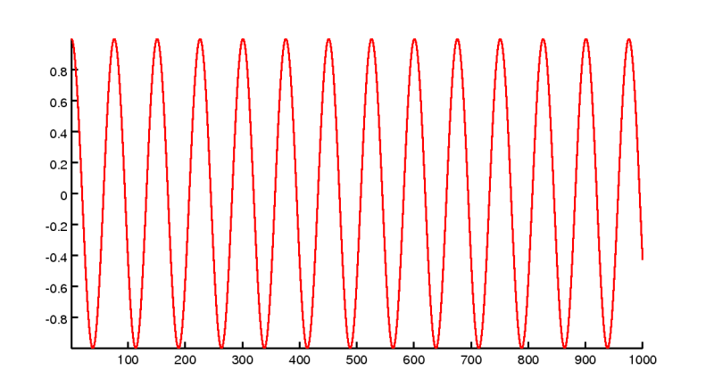
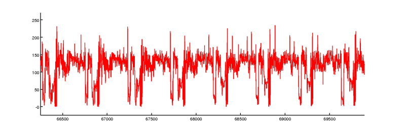
If you don’t believe my derivation, maybe you believe a (modified) function plot:

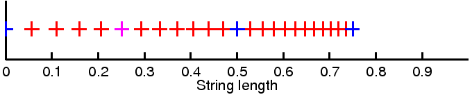
The blue crosses indicate the first two octaves, occurring when ½ (=50%) and ¾ (=75%) of the length are removed. The pink cross indicates the fifth fret at about ¼ (=25.085%) of the length. Every guitarist should recognize the fret stepping here!

Gauge stepping when tuning down
I found a link which explains that the relation between string diameter δ, tension t and frequency f is

,

where C is a constant depending on the material. The aforementioned scaling is still valid for the frequencies, i.e., when the frequency f is tuned down by n halftones, the resulting frequency f_n is given as

,

what can be verified for f=440Hz: The next lower tunes are 415.3Hz (n=1) and 392Hz (n=2), and the next higher tunes are 466.2Hz (n=−1) and 493.9Hz (n=−2). Replacing f by f_n in the previous equation yields that when the tension is to be kept, one has to take strings with diameter . As example, .009’er strings that are tuned down by one whole tone should be replaced by .010’ers to keep the tension of the .009’ers.

The other way round, fixing δ_n=0.010 (the taken string gauge) and δ=0.009 (the desired string gauge “feel”), one derives

what results in n=1.82 in this example, a downtune of slightly less than a whole tone. Tuning down .010’ers a “complete” whole tone corresponds to a string gauge of .0089’ers, so really almost .009’ers.

As a final rule of thumb, the steps between the string gauges correspond to tune changes of a whole tone. The following table shows how certain string gauges “feel” when they are tuned down:

tuning	.008	.009	.0095	.010	.011	.012	.013
E♭	.0076	.0085	.009	.0094	.0104	.0113	.0123
D	.0071	.008	.0085	.0089	.0098	.0107	.0116
D♭	.0067	.0076	.008	.0084	.0092	.010	.011
C	.0063	.0071	.0075	.0079	.0087	.0095	.0103
B	.006	.0067	.0071	.0075	.0082	.009	.0097

Given an image im of size p×q with gcd(p,q)=1.

• Find a number s that is not divided by the divisors of N=pq.
• Index vector, method 1:
• idx = mod(1:s:N*s, N);
• nil = find(idx==0); idx(nil)=N;
• Index vector, method 2 (preferred):
• idx = mod((1:s:N*s)-1, N)+1;
• imv(idx) = im(:);

Reconstruction from vector of length N=pq:

• rim = reshape(imv(idx), p, q);

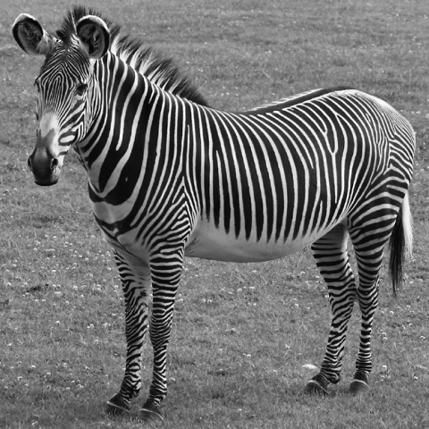
Let’s try this with our zebra. In my previous tries I simply took p=479 and q=480 to have gcd(479,480)=1, but 479 is a prime number and I therefore have no possibility to divide it by some step size. For GA I have to lay some kind of lattice over the image. So there is actually a second condition forbidding p and q to be prime. I take p=473 instead, it has 11 and 43 as divisors.

As one can see, N has many divisors, but e.g. 19 is not one of them. We can’t take e.g. 9 although it doesn’t occur either, as it is divided by 3, which is a divisor of N. Taking such a wrong step size will lead one back to the first pixel too early and one can never span the whole image.

And now the other way round:

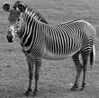
Indeed looks like our zebra!

By the way, another try of comparing the FFT of the vector with the FFT2 of the image shows again that one cannot get the FFT2 by doing an FFT of the vector. This is because the line-patterns in the image might not be preserved under that transform, as neighboring pixels might not become neighbors in the resulting vector.

I found a quicker way to compute the index matrix I mentioned: So nothing with 58 seconds anymore.

Regarding the previous questions I noticed that GA on LCA groups is too general for my concerns and that the study of GA on finite abelian groups is enough.

In a certain paper HGFei published a result that for p×q-images where p and q are relatively prime there is an isomorphism to a vector of length N=pq. The theory considers the groups and where . One explicit mapping from the matrix indices to the corresponding vector indices is given by

where α and β are integers chosen such that

My 480×480 zebra-image doesn’t have a height and width that are relatively prime, so I simply drop one pixel of height:

Just for a first test I set α=p and β=q and define a primitive mapping function. (I’ll have to find a quicker transform, as in my tests the switching takes too long. But this could be due to the actually large test image. In addition, I currently only manage to do the backward step by storing the indices in an index matrix.)

I have to return N instead of 0 to have a correct index value. Although the mapping is actually an isomorphism I didn’t know how to go back to the tuple (j,k), so I store the indices in an index matrix while building the image vector:

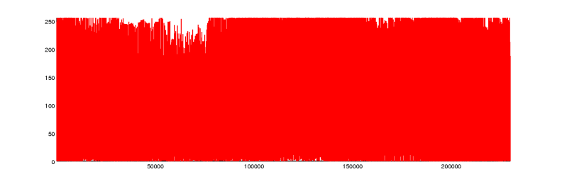
58 seconds!? However, the image looks like this as a vector:

I noticed that I’ll have to find a representation of images as vectors, and not as matrices as usual. Because otherwise I won’t be able to describe linear operations as matrices on vectors. To be able to do things like an SVD or a look at eigenvalues or eigenvectors, I’ll have to evaluate matrices on vectors. For building lattices or Gabor systems I’ll have to try to use the algorithms which have been developed for 1D-signals. This leads me to Gabor Analysis on locally compact abelian groups, but group theory is a little bit away from ordinary signal analysis. Reading first intros, I asked myself:

70. What are compact groups? What are locally compact groups? What is a compactly generated group? What is an open compact subgroup?
    As an example, seems to be a compact group whenever A is real-valued invertible d×d. d=1 makes and a compact group.
71. What is a discrete (sub-)group? Why is the dual of a compact group discrete?
72. Why is for and a real-valued invertible d×d-matrix A?
    Maybe because for invertible square matrices and , and clearly .
73. How can I implement the tensor product of separable lattices to get non-separable lattices like the quincunx lattice or a hexagonal lattice?

I finally managed to scale the reconstructed images appropriately such that one can see at what locations certain 2D-frequencies occur. I FT’ed an image of a zebra and “windowed” the FT with a shifted Gaussian. Doing the inverse FT of that cutout yields a convolution of the input image with a modulated Gaussian, corresponding to

This is the zebra, a 480×480 pixel sample I clipped from an image I found in the Wikimedia Commons, and its FFT2:

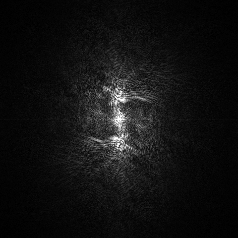
Again, I rotated the image of the FT by 90° to match the orientation of the “jets” with the line patterns in the zebra. Clearly, the vertically oriented frequencies dominate the image. Now I window the FT-image by placing a Gaussian at the origin. This results in a low-pass filter. The IFT gives a reconstructed image which only contains the lowest frequencies:

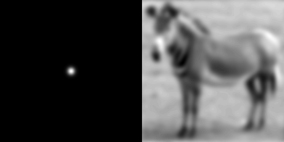
The left half shows the (unmodulated) Gaussian with which the original image has been convolved. The right half shows the reconstructed image—the animal has lost all its zebra patterns! This effect is identical to a Gaussian blur.