I always wondered why it didn’t work to compute the dual Gabor atom by using the image-to-vector methods I explained previously [1,2,3]. Dr. Kaiblinger showed me that the correct way was to use that special isomorphism that walks along the diagonal of the image. Because width and height have to be relatively prime, that path spans the whole image space. And because there are no jumps over pixels, 2D-modulations stay 1D-modulations. This is not yet proved formally, but I can already show first experiments:
> p=64; q=75; idx=linind(p,q); %index vector
> img=zeros(p,q); N=p*q
N = 4800
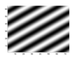
> img(idx(1:50))=1; imagesc(img); %step 50
> img(idx(1:100))=1; imagesc(img); %step 100
> img(idx(1:1000))=1; imagesc(img); %step 1000
> img(idx(1:4000))=1; imagesc(img); %step 4000
A 2D-frequency is given as a tensor product of two 1D-frequencies with signal lengths p and q, respectively. If their modulation parameters are given as kp and kq, then the corresponding 2D-modulation is given by a 1D-modulation of length N and parameter kN = kq p − kp q (mod N) ; as already said, a proof is not given yet.
> kp=4; frp = exp(2*pi*i*(0:p-1) * kp/p);
> kq=3; frq = exp(2*pi*i*(0:q-1) * kq/q);
> frpq = frp’ * frq; size(frpq)
ans =
64 75
> imagesc(real(frpq))
> kN = mod(kq*p-kp*q, N)
kN = 4692
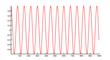
> frN = exp(2*pi*i*(0:N-1) * kN/N);
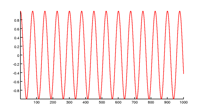
> plot(real(frN(1:1000)))
> frN2=zeros(p,q);
> frN2(idx)=frN;
> compnorm(frpq, frN2)
quotient of norms: norm(x)/norm(y) = 1
difference of normalized versions = 1.478e-12
ans = 1.4780e-12
So those two 2D-frequencies are really identical. The plot of the second one is identical to the first one, so we skip it here.
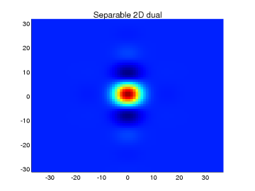
Now we want to see if the 2D-dual of a separable 2D atom obtained by that isomorphism is identical to the tensor product of the two 1D-duals.
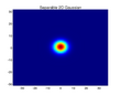
> gp=gaussnk(p); % Gaussian of length p
> gq=gaussnk(q); % Gaussian of length q
> g=gp’*gq; % tensor product
> imgc(g)
> title(’Separable 2D Gaussian’)
> alldiv(p)
ans =
2 4 8 16 32
> ap=4; bp=8; p/ap * p/bp / p % redundancy along p
ans = 2
> alldiv(q)
ans =
3 5 15 25
> aq=5; bq=5; q/aq * q/bq / q % redundancy along q
ans = 3
> gpd=ppdw(gp,ap,bp); % dual of gp
> gqd=ppdw(gq,aq,bq); % dual of gq
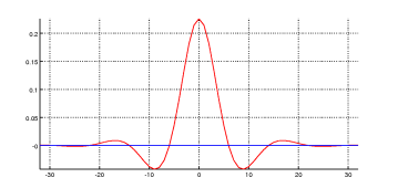
> plotc(gpd)
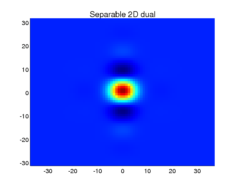
> gd=gpd’*gqd; % tensor product
> imgc(gd)
> title(’Separable 2D dual’)
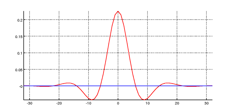
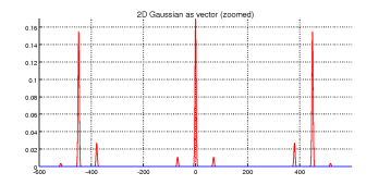
> gv=g(idx); % the 2D Gaussian as vector
> plotc(gv([1:600 N-600:N]))
> title(’2D Gaussian as vector (zoomed)’)
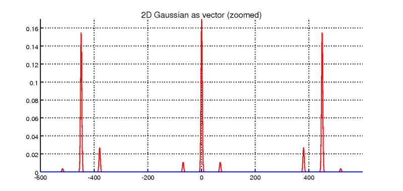
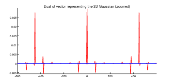
> gvd=ppdw(gv,ap*aq,bp*bq); % dual w/combined parameters
> plotc(gvd([1:600 N-600:N]))
> title(’Dual of vector representing the 2D Gaussian (zoomed)’)
> gd2=zeros(p,q);
> gd2(idx)=gvd; % reshaping to image matrix
> compnorm(gd,gd2)
quotient of norms: norm(x)/norm(y) = 1
difference of normalized versions = 2.439e-16
ans = 2.4390e-16
Indeed, both 2D duals are numerically identical, and a plot of the reshaped one looks identical to the one before.
A Gabor family can now be built by using the vector of the 2D atom, no matter if it was separable or not. However, it may become very large: In my example with a rather small image height of 64 and a width of 75 pixels, the combined 2D redundancy above was 6, so the Gabor matrix is of size 28,800×4,800, which already contains more than 138 million entries! Every single entry is of data type ‘double’ and therefore takes 8 bytes, so the whole Gabor matrix needs the huge memory space of more than 1GB! In this case one cannot compute the Gabor matrix explicitly, but at least one can compute the STFT using the 1D vector of the 2D window, because the 1D modulations correspond to 2D modulations as shown at the beginning.