Stephan Paukner :: syslog

I finally managed to scale the reconstructed images appropriately such that one can see at what locations certain 2D-frequencies occur. I FT’ed an image of a zebra and “windowed” the FT with a shifted Gaussian. Doing the inverse FT of that cutout yields a convolution of the input image with a modulated Gaussian, corresponding to

.

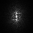
This is the zebra, a 480×480 pixel sample I clipped from an image I found in the Wikimedia Commons, and its FFT2:

Again, I rotated the image of the FT by 90° to match the orientation of the “jets” with the line patterns in the zebra. Clearly, the vertically oriented frequencies dominate the image. Now I window the FT-image by placing a Gaussian at the origin. This results in a low-pass filter. The IFT gives a reconstructed image which only contains the lowest frequencies:

The left half shows the (unmodulated) Gaussian with which the original image has been convolved. The right half shows the reconstructed image—the animal has lost all its zebra patterns! This effect is identical to a Gaussian blur.