Wednesday, November 15. 2006
The exponential in $R^d$, II

(Q15) I’m gonna show you some cool Gabor atoms on .
, as described previously, indeed looks like this:
[xx yy] = meshgrid(linspace(-2,2,100));
v=[1 1.5];
e1 = exp(pi*i*( v(1)*xx + v(2)*yy ));
imagesc(real(e1))
w=[-1 4];
e2 = exp(pi*i*( w(1)*xx + w(2)*yy ));
imagesc(real(e2))
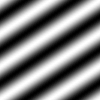

See how the value of the frequency changes with the length of , and the direction with the orientation of
, just as described previously.
In the STFT, these frequencies get reduced locally by an “envelope function”. One could take the Gaussian window to achieve this:
g1 = exp(-(xx.^2+yy.^2));
imagesc(g1)
g2 = exp(-4*(xx.^2+yy.^2));
imagesc(g2)

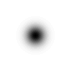
And now these are the modulated Gaussians, whose set of translates across forms the building blocks for Gabor analysis on
:
imagesc(real(g1.*e1))
imagesc(real(g2.*e2))


(Page 1 of 1, totaling 1 entries)
About
Calendar
Archives
Categories
Show tagged entries
android antenna anti-spam apache austria automobile ballooning bash bluetooth bug career cloud collecting cooking crypto cw debian diy dreams education electronics event fail fashion finance flickr fuerteventura fun gentoo geography german gnu-linux gnucash google google earth graphics guitar hardware history image processing internet kernel kids language lanzarote lhc lifestyle linkroll literature ltd machine learning making mallorca mathematics matlab migration munich music nautilus numismatics octave perl philately philosophy phone photo gear photography physics podcast politics postfix private programming public transport rant religion review salzburg samsung science security social web software statistics storage sustainability symbian tablet time lapse transceiver tv usenet venice video virtualization wordplay work www yahoo youtube