The exponential in $R^d$, II

Stephan Paukner :: syslog

Wednesday, November 15. 2006

The exponential in $R^d$, II

(Q15) I’m gonna show you some cool Gabor atoms on $\bbR^2$ . First, the function $u_\omega(x):=e^{\pi\i\langle x,\omega\rangle}$ , as described previously, indeed looks like this:

CODE:

[xx yy] = meshgrid(linspace(-2,2,100)); v=[1 1.5]; e1 = exp(pi*i*( v(1)*xx + v(2)*yy )); imagesc(real(e1)) w=[-1 4]; e2 = exp(pi*i*( w(1)*xx + w(2)*yy )); imagesc(real(e2))

See how the value of the frequency changes with the length of $\omega$ , and the direction with the orientation of $\omega$ , just as described previously.
In the STFT, these frequencies get reduced locally by an “envelope function”. One could take the Gaussian window $e^{-a^2x^2}$ to achieve this:

CODE:

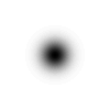
g1 = exp(-(xx.^2+yy.^2)); imagesc(g1) g2 = exp(-4*(xx.^2+yy.^2)); imagesc(g2)

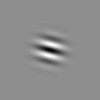
And now these are the modulated Gaussians, whose set of translates across $\bbR^2$ forms the building blocks for Gabor analysis on $\bbR^2$ :

CODE:

imagesc(real(g1.*e1)) imagesc(real(g2.*e2))

Posted by Stephan Paukner in Master's Thesis at 17:15 | Comments (0) | Trackback (1)

Defined tags for this entry: mathematics, matlab, octave

Trackbacks

Trackback specific URI for this entry

Logbook of Stephan Paukner on : Convolving a zebra with modulated Gaussians

I finally managed to scale the reconstructed images appropriately such that one can see at what locations certain 2D-frequencies occur. I FT&#8217;ed an image of a zebra and &#8220;windowed&#8221; the FT with a shifted Gaussian. Doing the inverse FT of th

Comments

Display comments as (Linear | Threaded)

No comments

Add Comment

Name

Homepage

Comment

In reply to

Phone*

What is three plus five?

Enclosing asterisks marks text as bold (*word*), underscore are made via _word_.

Standard emoticons like :-) and ;-) are converted to images.

To prevent automated Bots from commentspamming, please enter the string you see in the image below in the appropriate input box. Your comment will only be submitted if the strings match. Please ensure that your browser supports and accepts cookies, or your comment cannot be verified correctly.
CAPTCHA