Thursday, May 31. 2007
Review: Pirates Of The Caribbean III

Now I remember why I rarely go to the movies.
POTC (the first part) was a rather amusing film. But POTC2 was a lame sequel (like they usually are), and POTC3 was trash (like they usually are, see
You are what you eat

TV confusion
Five murder mystery TV shows with blondes in the lead and starting with “C”: C.S.I., Criminal Intent, The Closer, Close To Home, Cold Case.
No wonder I’m confused. And I always thought that TV is only for people with an
Wednesday, May 30. 2007
Separable vs. non-separable lattices

I used P. Prinz’ toolbox to compute a 2D dual atom on a separable lattice and on a quincunx lattice. It shows that even if both lattices have same redundancy, the dual might be better localized on the quincunx lattice:
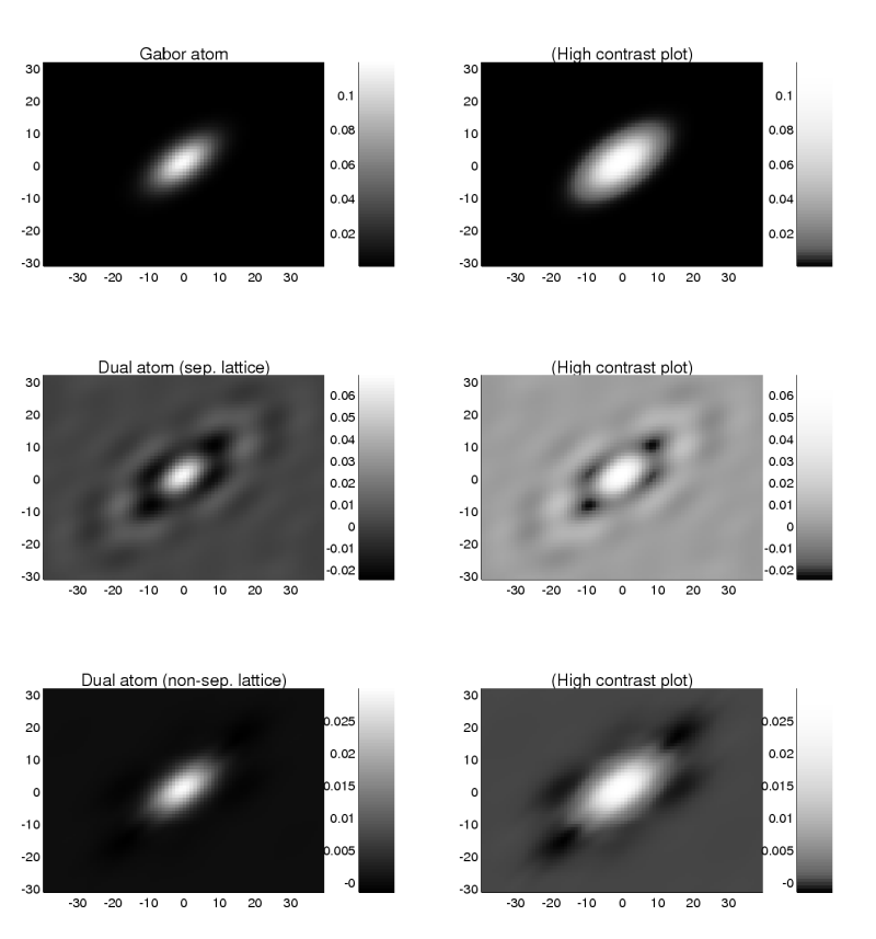
In this example, the norm difference of the “quincunx dual” to the original is about 0.1, and that between the “separable dual” and the original is almost 1.0. To achieve more similarity on the separable lattice, one has to take a higher redundancy.
I’m still not sure what the term “separability” actually expresses for 4D lattices: There exist position lattices (on the image space), frequency lattices (on the FT space), and TF-lattices (for both dimensions). If the atom is separable into its two dimensions, then one can compute the two 1D duals and obtain the 2D dual from their tensor product. If one takes two quincunxes for computing those two 1D duals, does this correspond to a non-separable 4D PF-lattice? In the case of 1D signals, a separable TF-lattice means that there’s always the same set of frequencies taken at every position. A quincunx lattice means that there are two different sets of frequencies chosen alternately while walking along the position points. Maybe the same interpretation works for the 2D case. I haven’t analyzed Prinz’ routine yet, but I think that he takes a rectangular (separable) frequency lattice and shifts it alternately by a half of the lattice-point distance while walking along the position spots. Should one try to use a quincunx position lattice? Well, I’ll have to experminent with that.
HGFei asked me to contact Søndergaard, because that topic of non-separability is currently not only “hot” for myself.
Friday, May 25. 2007
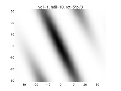
Dilated + rotated 2D Gaussian
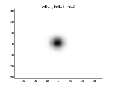
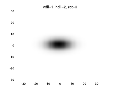
I’ve finally improved my script that computes a dilated and rotated 2D Gaussian with respect to low memory consumption. It applies a dilation and rotation matrix to the 2D domain. I published it under the GNU GPLv2, so if you find any improvements, you are forced to share them. 
I still have the impression that it is rather slow, but I currently don’t know how to do it better. Of course, it has to be evaluated on
% Computes a non-separable (dilated + rotated) 2D Gaussian
% Usage: g = nsgauss(p, q, vdil, hdil, rot);
% Input: p,q .... size of g
% vdil ... vertical dilation factor (before rotation)
% hdil ... horizontal dilation factor (before rotation)
% rot .... rotation angle, e.g. pi/4
% Example:
% norm(nsgauss(p,q,1,1,0) - gaussnk(p)’*gaussnk(q)) == eps
%
% Version 0.2-20070525
% by Stephan Paukner {stephan+math at paukner dot cc}
% Licensed under the GNU General Public License v2
% $Id: nsgauss.m,v 1.2 2007/05/25 10:14:52 ps Exp ps $
D=[1/vdil 0; 0 1/hdil]; %dilation matrix
R=[cos(rot) -sin(rot); sin(rot) cos(rot)]’; %’%rotation matrix
sp=sqrt(p); sq=sqrt(q);
g=zeros(1,p*q);
for jp=-3:3
for jq=-3:3
[x y]=meshgrid( (0:p-1)/sp + jp*sp , (0:q-1)/sq + jq*sq );
v=D*R*[x(:)’; y(:)’];
g=g+exp(-pi*(v(1,:).^2 + v(2,:).^2));
end
end
g=reshape(g,q,p)’; %’
g=g/norm(g,’fro’);
Here’s a comparison of computing time and accuracy:
And some plots using different parameters:
 |  |
 |  |
 |  |
Storage capacity consideration

In my notebook, I have a 60GB disk, 27+14=41GB considered for the whole Linux system and 11.5GB left for various personal files. In my backup PC, I have a 112GB /home partition (LVM on RAID-5) and 12GB left, another 12GB are available on the /usr partition and 8.6GB in /opt, and as everything is on LVM, it might be resizable. So there’s currently no real need for additional disk space. The only drawback is that I can’t hold all music files on my notebook and that the available space is splitted into two partitions. But I can live with that, I just have to consider that some things will be in a mounted subdirectory.
When space will get small, I’ll buy a 160GB notebook-disk. And my backup PC will be a new one with two 500GB SATA-disks on RAID-1. I won’t take a kind of commercial network storage array, as these aren’t capable of rsync or the like.
I thought about taking RAID-5 again instead of RAID-1. Three 320GB disks are cheaper than two with 500GB, but data redundancy decreases from 2 to 1.5. Only one disk may fail in both cases, no matter if you’ve got two disks at RAID-1 or three disks at RAID-5. In addition, the probability that two disks fail is three(!) times higher when there are three disks as if there were only two. For me, RAID-5 is therefore just a strategy for expansion, not for starting freshly.
Monday, May 21. 2007
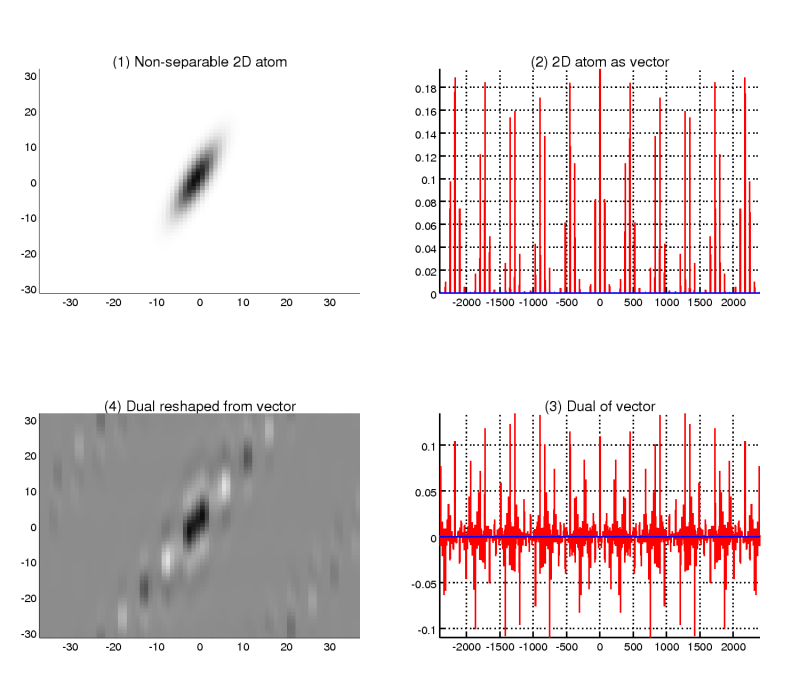
2D dual via 1D dual
Yesterday I finally wrote a routine which computes a non-separable (dilated and rotated) 2D Gaussian. It takes parameters for horizontal and vertical dilation of the 2D Gaussian which is then rotated by a corresponding parameter. If it is neither dilated nor rotated, it is numerically identical to the pure 2D Gaussian. It has
With this I could finally reproduce a graphic from the paper “2D-GA Based on 1D Algorithms”: It shows (1) a non-separable 2D atom with relatively prime height and width, (2) the atom mapped to vector shape, (3) the dual of that vector with regard to some combined time and frequency steps, and (4) the dual vector reshaped to an image.
The question remains about how to finally do GA using these two 2D atoms. The only ways I found so far was either building the 1D Gabor system (of the atom shaped as vector) or computing a sampled STFT by that 1D vector; this works because modulations stay modulations. However, in the case of separable 2D atoms, this can be done in another way, as I’ll show in another article.
Friday, May 18. 2007
Images to vectors: Correct isomorphism
I always wondered why it didn’t work to compute the dual Gabor atom by using the image-to-vector methods I explained previously [1,2,3]. Dr. Kaiblinger showed me that the correct way was to use that special isomorphism that walks along the diagonal of the image. Because width and height have to be relatively prime, that path spans the whole image space. And because there are no jumps over pixels, 2D-modulations stay 1D-modulations. This is not yet proved formally, but I can already show first experiments:
 Step 50 |  Step 100 |  Step 1000 |  Step 4000 |
A 2D-frequency is given as a tensor product of two 1D-frequencies with signal lengths p and q, respectively. If their modulation parameters are given as kp and kq, then the corresponding 2D-modulation is given by a 1D-modulation of length N and parameter

So those two 2D-frequencies are really identical. The plot of the second one is identical to the first one, so we skip it here.
Now we want to see if the 2D-dual of a separable 2D atom obtained by that isomorphism is identical to the tensor product of the two 1D-duals.
Continue reading "Images to vectors: Correct isomorphism"